Find The Best Distribution For Your Data
MAADSBML has a powerful functionality to find the best distribution for your data. Meaning, it will apply analyse your data and iterate through complex distributions to find the one that BEST fits your data.
Important
Knowing the distribution of your data is critical for machine learning. Specifically, knowing the distribution is important for:
calculating the critical regions for hypothesis testing and confidence intervals
Machine learning algorithms are often based on distributional assumptions and violating these assumptions can lead to biased results
Helps in the choice of algorithms to use
How To Find The Best Distribution
MAADSBML has a function called: finddistribution. Refer to MAADSBML Python Library API
This is a powerful yet simple function to use. With ONE-LINE of code, MAADSBML will find the best distribution for your data in seconds.
Here are all the distributions it will analyse for your data, and choose the BEST one using the sumsquare_error method, see Outputs: Comprehensive JSON Data File
Important
The distribution with the lowest sumsquare_error is the BEST one. using the sumsquare_error method, see Outputs: Comprehensive JSON Data File
[‘alpha’, ‘anglit’, ‘arcsine’, ‘argus’, ‘beta’, ‘betaprime’, ‘bradford’, ‘burr’, ‘burr12’,
‘cauchy’, ‘chi’, ‘chi2’, ‘cosine’, ‘crystalball’, ‘dgamma’, ‘dweibull’, ‘erlang’, ‘expon’,
‘exponnorm’, ‘exponpow’, ‘exponweib’, ‘f’, ‘fatiguelife’, ‘fisk’, ‘foldcauchy’, ‘foldnorm’,
‘frechet_l’, ‘frechet_r’, ‘gamma’, ‘gausshyper’, ‘genexpon’, ‘genextreme’, ‘gengamma’,
‘genhalflogistic’, ‘geninvgauss’, ‘genlogistic’, ‘gennorm’, ‘genpareto’, ‘gilbrat’, ‘gompertz’,
‘gumbel_l’, ‘gumbel_r’, ‘halfcauchy’, ‘halfgennorm’, ‘halflogistic’, ‘halfnorm’,
‘hypsecant’, ‘invgamma’, ‘invgauss’, ‘invweibull’, ‘johnsonsb’, ‘johnsonsu’, ‘kappa3’, ‘kappa4’,
‘ksone’, ‘kstwo’, ‘kstwobign’, ‘laplace’, ‘levy’, ‘levy_l’, ‘levy_stable’, ‘loggamma’, ‘logistic’,
‘loglaplace’, ‘lognorm’, ‘loguniform’, ‘lomax’, ‘maxwell’, ‘mielke’, ‘moyal’, ‘nakagami’, ‘ncf’,
‘nct’, ‘ncx2’,‘norm’, ‘norminvgauss’, ‘pareto’, ‘pearson3’, ‘powerlaw’, ‘powerlognorm’, ‘powernorm’,
‘rayleigh’, ‘rdist’, ‘recipinvgauss’, ‘reciprocal’, ‘rice’, ‘rv_continuous’, ‘rv_histogram’,
‘semicircular’, ‘skewnorm’, ‘t’, ‘trapz’, ‘triang’, ‘truncexpon’, ‘truncnorm’, ‘tukeylambda’,
‘uniform’, ‘vonmises’, ‘vonmises_line’, ‘wald’, ‘weibull_max’, ‘weibull_min’, ‘wrapcauchy’]
How To Use finddistribution Function
The best way is to learn this function is by an example. In the code below, you can test this function for yourself and see its power.
The code can be found here on GitHub
The data files are also here on GitHub
import maadsbml
import numpy as np

def finddist(filename,varname,dataarr,folderpath,imgname,fast=1,topdist=6):
    status,dist,bestdist,alldata=maadsbml.finddistribution(filename,varname,dataarr,folderpath,imgname,fast,topdist)
    print(status)

def genarray():
    mu, sigma = 1, 10.5 # mean and standard deviation
    data = np.random.normal(mu, sigma, 100)
    return data

# Example File 1
filename="body_fat.csv"
# The variable for distributional analysis in body_fat.csv
varname="%Fat"
# Example file 2
filename="weight_height.csv"
# The variable for distributional analysis in weight_height.csv
varname="Height"
# Folder path to save output.  Enter valid path, or it will be saved in current directory.
folderpath='.'
# name of file
imgname="bml"

# We will generate a random array for distributional analysis but we could comment this out and use the above files or any other data
dataarr = genarray()
varname="Sample Data"
# here we are using 1 for FAST distribution analysis using the most common distributions
# 7 to print the TOP 7 distributions in the image and JSON
# Use either filename or dataarr NOT both
filename=""
try:
 finddist(filename,varname,dataarr,folderpath,imgname,1,7)
except Exception as e:
  print(e)
Outputs From finddistribution
The output of the finddist function will be:
Outputs: Four Returned Variables
FOUR return variable:
status: will indicate any ERROR success
dist: distribution dataframe
bestdist: name of best distribution
alldata: comprehensive JSON data file
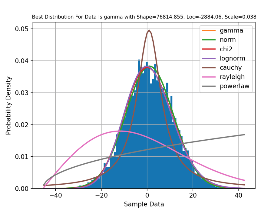
Outputs: Distribution Image
Image of your distribution curve mapped to your data, as shown below (showing the TOP 7 BEST distributions): See output image here on GitHub
Outputs: Comprehensive JSON Data File
JSON file (same as alldata): See Output Here on GitHub
A summary of the results is also contained in the JSON file. Specifically, gamma is the BEST distribution based on the lowest sumsquare_error = 0.0001814887:
"summary": {
        "sumsquare_error": {
                "gamma": 0.0001814887,
                "norm": 0.0001828346,
                "chi2": 0.0002025934,
                "lognorm": 0.0002224293,
                "cauchy": 0.0027350555,
                "rayleigh": 0.0117642895,
                "powerlaw": 0.017502358
        },
        "aic": {
                "gamma": 1265.1777664529,
                "norm": 1262.325861669,
                "chi2": 1295.9483921464,
                "lognorm": 1322.0959274175,
                "cauchy": 1064.0702058171,
                "rayleigh": 943.187532113,
                "powerlaw": 920.517365162
        },
        "bic": {
                "gamma": 1286.8087875688,
                "norm": 1276.746542413,
                "chi2": 1317.5794132623,
                "lognorm": 1343.7269485335,
                "cauchy": 1078.4908865611,
                "rayleigh": 957.6082128569,
                "powerlaw": 942.148386278
        },
        "ks_statistic": {
                "gamma": 0.0081781542,
                "norm": 0.0086574911,
                "chi2": 0.0119634473,
                "lognorm": 0.0146829697,
                "cauchy": 0.0741439895,
                "rayleigh": 0.2884171645,
                "powerlaw": 0.3436579581
        },
        "ks_pvalue": {
                "gamma": 0.5128041638,
                "norm": 0.4392613156,
                "chi2": 0.1133222869,
                "lognorm": 0.0265547382,
                "cauchy": 2.970808383e-48,
                "rayleigh": 0.0,
                "powerlaw": 0.0
        }
},
"filename": "",
"varname": "Sample Data",
"folderpath": ".",
"distimagefilename": "bml.png",
"jsondatafilename": "bml.json",
"nobs": 10000,
"min": -45.517,
"max": 42.882,
"mean": 1.035,
"variance": 108.372,
"std": 10.41,
"skewness": 0.007,
"kurtosis": 0.045,
"isarray": 1